Solving the Laplace Equation on GPU with OpenACC

Pre-requisites

Ensure you are able to connect to the UL HPC cluster. In particular, recall that the module command is not available on the access frontends.

Access to the ULHPC iris cluster (here it is the only one featuring GPU nodes):

(laptop)$> ssh iris-cluster

/!\ Advanced (but recommended) best-practice: Always work within a GNU Screen session named with 'screen -S ' (Adapt accordingly) IF not yet done, copy ULHPC .screenrc in your home:

(access)$> cp /etc/dotfiles.d/screen/.screenrc ~/

Now, you need to pull the latest changes in your working copy of the ULHPC/tutorials you should have cloned in ~/git/github.com/ULHPC/tutorials (see "preliminaries" tutorial)

(access)$> cd ~/git/github.com/ULHPC/tutorials
(access)$> git pull

Access to a GPU-equipped node of the Iris cluster

This practical session assumes that you have reserved a node on iris with one GPU for interactive development. See documentation

### Have an interactive GPU job
# ... either directly
(access)$> si-gpu
# ... or using the HPC School reservation 'hpcschool-gpu' if needed - use 'sinfo -T' to check if active and its name
# (access)$> si-gpu --reservation=hpcschool-gpu
$ nvidia-smi

Objectives

This tutorial aims to show how the OpenAcc directives can be used to accelerate a numerical solver commonly used in engineering and scientific applications. After completing the exercise of this tutorial, you would be able to:

Transfer data from the host to device using the data directives,
Accelerate a nested loop application with the loop directives, and,
Use the reduction clause to perform summation on variables or elements of a vector.

The Laplace Equation

The Laplace differential equation in 2D is given by:

$\nabla^2 F = \frac{d^2F}{dx^2} + \frac{d^2F}{dy^2} = 0$

It models a distribution at steady-state or equilibrium in a 2D space (e.g., Temperature Distribution).
The Laplace differential equation can be solved using the Jacobi method if the boundary conditions are known (e.g., the temperature at the edges of the physical region of interest)

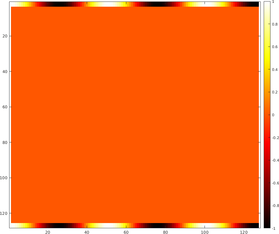
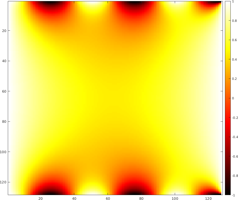
An example of a 2D problem is demonstrated in the figures below. The first figure presents the temperature at the edges of a plane. The solution of the Laplacian equation providing the steady-state temperature distribution was calculated for the given boundary condition using the Jacobi method and is shown in the second figure.

Boundary Conditions

Solution

The Jacobi method

Iterative method for solving a system of equations:

$Ax = b$

where, the elements $A$ and $b$ are constants, and $x$ is the vector with the unknowns.

At each iteration, the elements $x$ are updated using their previous estimations by:

$x_i = \frac{1}{A_{ii}}(b_i - \sum_{i \ne j} A_{ij}x^{k-1}_j)$

An error metric is calculated at each iteration $k$ over the elements $x_i$ :

$Error = \sum_i (x^k_i - x^{(k-1)}_i)^2$

The algorithm terminates when the error value becomes smaller than a predefined threshold:

$Error<Threshold$

Solving the Laplace Equation using the Jacobi method

Second-order derivatives can be calculated numerically for a small enough value of $\delta$ by:

$\frac{d^2F}{dx^2} = \frac{1}{\delta ^2}(f(x+\delta, y) - 2f(x,y)+f(x-\delta,y))$

$\frac{d^2F}{dy^2} = \frac{1}{\delta ^2}(f(x, y +\delta) - 2f(x,y)+f(x, y-\delta))$

Substituting the numerical second-order derivatives in the Laplace equation gives:

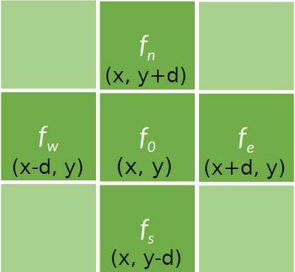
$f(x,y) = \frac{1}{4}(f(x, y +\delta) + f(x, y -\delta) + f(x+\delta, y) + f(x-\delta, y))$

The above equation results in a stencil pattern where the new value of an element is calculated using its neighbors. A stencil of four points is shown in the figure below. The Jacobi iterative method can lead to the solution of the Laplace equation by successively calculating the above stencil output for each element $f_i$ in the vector of unknowns which in this case is the vectorized representation of the examined distribution $F$ (e.g Temperature distribution) .

Stencil of 4 points

Serial Implementation of the Jacobi Method in C

A serial code implementing the Jacobi method employs a nested loop to compute the elements of a matrix at each iteration. At each iteration, the error value (distance metric) is calculated over these elements. This calculated error value is monitored in the main loop to terminate the iterative Jacobi algorithm.

while ((iter < miter )&& (error > thres))
{
error = calcTempStep(T, Tnew, n, m);

update(T, Tnew, n, m);

if(iter % 50 == 0) printf("Iterations = %5d, Error = %16.10f\n", iter, error);

iter++;
}

The nested loop is implemented in function calcTempStep(float *restrict F, float *restrict Fnew, int n, int m). n and m are the dimensions of the 2D matrix $F$ , $F$ is a vector containing the current estimations, and $F_{new}$ is a buffer storing the new elements' values as resulted from the stencil calculations. The error value is calculated for each new stencil calculation using the corresponding elements of vectors $F$ and $F_{new}$ . The error is summed (reduced) for all elements and returned to the function main.

float calcTempStep(float *restrict F, float *restrict Fnew, int n, int m)
{
float Fu, Fd, Fl, Fr;
float error = 0.0;


for (int i = 1; i < n-1; i++){
for (int j = 1; j < m-1; j++){
Fu = F[(i-1)*m + j];
Fd = F[(i+1)*m + j];
Fl = F[i*m + j - 1];
Fr = F[i*m + j + 1];
Fnew[i*m+j] = 0.25*(Fu + Fd + Fl + Fr);
error += (Fnew[i*m+j] - F[i*m+j])*(Fnew[i*m+j] - F[i*m+j]);
}
}


return error;
}

The function update(float *restrict F, float *restrict Fnew, int n, int m) implements a nested loop which is used to update the current estimates of $F$ with the stencil calculations stored in $F_{new}$ .

void update(float *restrict F, float *restrict Fnew, int n, int m)
{

for (int i = 0; i < n; i++)
for (int j = 0; j < m; j++ )
F[i*m+j] = Fnew[i*m+j];


}

Exercise:

Parallelize the Jacobi iteration with OpenACC

Follow the steps below to accelerate the Jacobi solver using the OpenAcc directives.

Task 1: If you do not yet have the UL HPC tutorial repository, clone it. Update to the latest version.

ssh iris-cluster
mkdir -p ~/git/github.com/ULHPC
cd ~/git/github.com/ULHPC
git clone https://github.com/ULHPC/tutorials.git
cd tutorials/gpu/openacc/laplace/exercise
git stash && git pull -r && git stash pop

Task 2: Get an interactive GPU job on iris cluster:

### ... either directly - dedicate 1/4 of available cores to the management of GPU card
$> si-gpu -c7
# /!\ warning: append -G 1 to reserve a GPU
# salloc -p interactive --qos debug -C gpu -c7 -G 1 --mem-per-cpu 27000

### ... or using the HPC School reservation 'hpcschool-gpu'
salloc --reservation=hpcschool-gpu -p interactive -C gpu --ntasks-per-node 1 -c7 -G 1

Task 3: Load the required modules:

module load compiler/PGI/19.10-GCC-8.3.0-2.32
module load compiler/GCC

Task 4: Use the source file jacobi.c under the folder OpenAccExe/exercise/ with your favorite editor (e.g. emacs). The C code implementing the method is already developed. Use the data directive to copy T and Tnew vectors in device memory before the loop in the function main:

//Code Here ! (1 line)
while ((iter < miter )&& (error > thres))
{
error = calcTempStep(T, Tnew, n, m);

update(T, Tnew, n, m);

if(iter % 50 == 0) printf("Iterations = %5d, Error = %16.10f\n", iter, error);

iter++;
}

Task 5: Use the parallel loop directive to parallelize the nested loop in function calcTempStep. Use a reduction clause (sum) to sum over the error values calculated for the pairs of elements T[i*m+j] and Tnew[i*m+j]:

float calcTempStep(float *restrict F, float *restrict Fnew, int n, int m)
{
float Fu, Fd, Fl, Fr;
float error = 0.0;

//Code Here! (1 line)
for (int i = 1; i < n-1; i++){
//Code Here! (1 line)
for (int j = 1; j < m-1; j++){
Fu = F[(i-1)*m + j];
Fd = F[(i+1)*m + j];
Fl = F[i*m + j - 1];
Fr = F[i*m + j + 1];
Fnew[i*m+j] = 0.25*(Fu + Fd + Fl + Fr);
error += (Fnew[i*m+j] - F[i*m+j])*(Fnew[i*m+j] - F[i*m+j]);
}
}


return error;
}

Task 6: Use the parallel loop directive to parallelize the nested loop in function update:

void update(float *restrict F, float *restrict Fnew, int n, int m)
{
//Code Here! (1 line)
for (int i = 0; i < n; i++)
//Code Here! (1 line)
for (int j = 0; j < m; j++ )
F[i*m+j] = Fnew[i*m+j];


}

Task 6: Compile and run your code

The PGI compiler 'pgcc' can be used to compile the source code containing OpenAcc directives. The -acc flag is required to enable the OpenAcc directives. The target architecture (Nvidia in this case) is defined using the -ta flag:

pgcc -acc -ta=nvidia -Minfo jacobi.c -o $exe

The compilation output indicates the part of the code that has been parallelized with the OpenAcc directives and provides information on the data transfers between the host and device. An example compilation output is given below:

calcTempStep:
41, Generating copyin(F[:n*m]) [if not already present]
Generating Tesla code
42, #pragma acc loop gang /* blockIdx.x */
Generating reduction(+:error)
44, #pragma acc loop vector(128) /* threadIdx.x */
Generating reduction(+:error)
41, Generating implicit copy(error) [if not already present]
Generating copyout(Fnew[:n*m]) [if not already present]
42, FMA (fused multiply-add) instruction(s) generated
44, Loop is parallelizable
update:
65, Generating copyin(Fnew[:n*m]) [if not already present]
Generating copyout(F[:n*m]) [if not already present]
Generating Tesla code
67, #pragma acc loop gang /* blockIdx.x */
69, #pragma acc loop vector(128) /* threadIdx.x */
69, Loop is parallelizable
Memory copy idiom, loop replaced by call to __c_mcopy4
main:
127, Generating copy(Tnew[:m*n],T[:m*n]) [if not already present]

To run the executable file interactively, use:

./$exe

where, $exe is the name of the executable after compilation. After running the script, the program prints to the screen the calculated error value at each iteration:

Iterations = 0, Error = 191.4627685547
Iterations = 50, Error = 0.3710202873
Iterations = 100, Error = 0.1216623262
Iterations = 150, Error = 0.0623667538
Iterations = 200, Error = 0.0387549363
Iterations = 250, Error = 0.0268577076
Iterations = 300, Error = 0.0199674908
Iterations = 350, Error = 0.0155865224
Iterations = 400, Error = 0.0126058822
Iterations = 450, Error = 0.0104726302
Iterations = 500, Error = 0.0088840043
Iterations = 550, Error = 0.0076624807
Iterations = 600, Error = 0.0066990838

The total time and number of iterations required for reducing the error value below the threshold value is printed when the program finishes its execution:

Total Iterations = 10000
Error = 0.0000861073
Total time (sec) = 2.976

Task 7: Compile and run the code without using the OpenAcc directives. This task can be performed by just compiling the code without using the -acc and -ta=nvidia flags:

pgcc -Minfo jacobi.c -o $exe

Run the serial application. What you observe? What is the acceleration achieved using the OpenAcc directives?