![]()
![]()

![]()
![]()

MATLAB (interactive, passive and sequential jobs) execution on the UL HPC platform
Copyright (c) 2013-2019 UL HPC Team <hpc-sysadmins@uni.lu>

The objective of this tutorial is to exemplify the execution of MATLAB - a high-level language and interactive environment for numerical computation, visualization and programming, on top of the UL HPC platform.
The tutorial will show you:
- how to run MATLAB in interactive mode, with either the full graphical interface or the text-mode interface
- how to check the available toolboxes and licenses used
- how to run MATLAB in passive (batch) mode, enabling unattended execution on the clusters
- how to use MATLAB script (.m) files
- how to plot data, saving the plots to file
- how to take advantage of some of the paralelization capabilities of MATLAB to speed up your tasks
For the tutorial we will use the UL HPC Iris cluster that includes nodes with GPU accelerators.
Prerequisites
As part of this tutorial two Matlab example scripts have been developed and you will need to download them, along with their dependencies, before following the instructions in the next sections:
    (access-iris)$> mkdir -p ~/matlab-tutorial/code
    (access-iris)$> cd ~/matlab-tutorial/code
    (access-iris)$> wget --no-check-certificate https://raw.github.com/ULHPC/tutorials/devel/maths/matlab/basics/code/example1.m
    (access-iris)$> wget --no-check-certificate https://raw.github.com/ULHPC/tutorials/devel/maths/matlab/basics/code/example2.m
    (access-iris)$> wget --no-check-certificate https://raw.github.com/ULHPC/tutorials/devel/maths/matlab/basics/code/google_finance_data.m
    (access-iris)$> wget --no-check-certificate https://raw.github.com/ULHPC/tutorials/devel/maths/matlab/basics/code/file_data_source.m
    (access-iris)$> wget --no-check-certificate https://raw.github.com/ULHPC/tutorials/devel/maths/matlab/basics/code/AAPL.csv
Or simply clone the full tutorials repository and make a link to this part of the MATLAB tutorial:
    (access-iris)$> git clone https://github.com/ULHPC/tutorials.git
    (access-iris)$> ln -s tutorials/maths/matlab/basics ~/matlab-tutorial
Matlab execution in interactive mode
Launching the full graphical environment
Running the full MATLAB environment on the Iris cluster will require you to enable X11 forwarding in order for the graphical environment to be shown on your local machine:
-
on Linux simply follow the commands below
-
on OS X (depending on version) you may not have the X Window System installed, and thus will need to install XQuartz if the first command below returns an 'X11 forwarding request failed on channel 0' error
-
on Windows you will either need to use MobaXTerm or if you use Putty, run VcXsrv first then configure Putty (Connection -> SSH -> X11 -> Enable X11 forwarding) before logging in to Iris.
# Connect to Iris with X11 forwarding enabled (Linux/OS X):
(yourmachine)$> ssh yourlogin@access-iris.uni.lu -p 8022 -X

# Request an interactive job (the default parameters get you 1 core for 2 hours) with an X11 tunnel:
(access-iris)$> salloc -p interactive bash -c 'ssh -X $(scontrol show hostnames | head -n 1)'

# Check the Matlab versions installed on the clusters:
(node)$> module avail matlab

# Load a specific MATLAB version:
(node)$> module load base/MATLAB/2018a

# Check that its profile has been loaded and thus we can start to use it:
(node)$> module list

# Launch MATLAB
(node)$> matlab
After a delay, the full Matlab interface will be displayed on your machine and you will be able to run commands, load and edit scripts and generate plots. An alternative to the graphical interface is the command-line (text-mode) interface, which is enabled through specific parameters, described in the following section.
Note: to request a full Iris node for a large interactive experiment you can:
-
Use all 28 cores within a node from the interactive partition, with 4GB RAM/core
salloc -p interactive -N 1 -n 1 -c 28 bash -c 'ssh -X $(scontrol show hostnames | head -n 1)' -
Use all 112 cores within a node from the bigmem partition, with ~27GB RAM/core
salloc -p bigmem -N 1 -n 1 -c 112 bash -c 'ssh -X $(scontrol show hostnames | head -n 1)'
Launching the command-line environment
Running the text-mode MATLAB interface in an interactive session, is much faster than using the full graphical environment through the network and is useful for commands/scripts testing and quick executions:
    # Connect to Iris, start an interactive job with 14 cores for 1 hour:

    (yourmachine)$> ssh yourlogin@access-iris.uni.lu -p 8022
    (access-iris)$> si -n 1 -c 14 --time 1:0:0
    (node)$> module load base/MATLAB/2018a

    # Launch MATLAB with the graphical display mode disabled (critical parameters):
    (node)$> matlab -nodisplay -nosplash
    Opening log file:  /home/users/vplugaru/java.log.46818

                                   < M A T L A B (R) >
                         Copyright 1984-2018 The MathWorks, Inc.
                          R2018a (9.4.0.813654) 64-bit (glnxa64)
                                    February 23, 2018

    To get started, type one of these: helpwin, helpdesk, or demo.
    For product information, visit www.mathworks.com.

    >> version()
    ans =
        '9.4.0.813654 (R2018a)'
In this command line you are now able to run Matlab commands, load and edit scripts, but cannot display plots - they can
however be generated and exported to file, which you will need to transfer to your own machine for visualisation.
While the text mode interface is spartan, you still benefit from tab-completion (type the first few letters of
a command then press TAB twice to see possible completions) and can run the integrated help with help command_name
(e.g. help plot3).
Example usage of Matlab in interactive mode
At this point you should have downloaded the example scripts and started Matlab either with the graphical or the text-mode interface. We will now test some Matlab commands by using the google_finance_data function defined in google_finance_data.m. This function downloads stock market data through the Google Finance API, and we will use it to get 1 month worth of stock data for IBM (whose stock symbol is 'IBM'):
     >> cd('~/matlab-tutorial/code/')
     >> [hist_date, hist_high, hist_low, hist_open, hist_close, hist_vol] = google_finance_data('IBM', '2017-05-01', '2017-06-02');
     >> size(hist_date)
     ans =
         24     1
     >> [hist_date{1} ' ' hist_date{end}]
     ans =
         '1-May-17 2-Jun-17'
     >> min(hist_low)
     ans =
       149.7900
     >> max(hist_high)
     ans =
       160.4200
     >> mean(hist_close)
     ans =
       153.2879
     >> std(hist_close)
     ans =
         2.7618
Note: If the Google Finance API is not available, you can use the file_data_source.m function with the AAPL ticker to use pre-downloaded data.
Through these commands we have seen that the function returns column vectors, we were able to get 24 days' worth of information and we used simple statistic functions to get an idea of how the stock varied in the given period.
Now we will use the example1.m script that shows: - how to use different plotting methods on the data retrieved with the google_finance_data function - how to export the plots in different graphic formats instead of displaying them (which is only available when running the full graphical environment and also allows the user to visually interact with the plot)
     >> example1
     Elapsed time is 1.709865 seconds.
     >> quit
     (node)$>
     (node)$> ls *pdf *eps
     example1-2dplot.eps  example1-2dplot.pdf  example1-scatter.eps
Note: You'll need to edit example1.m to use the offline data source file_data_source.m in place of the Google Finance API, if running example1 shows an error.
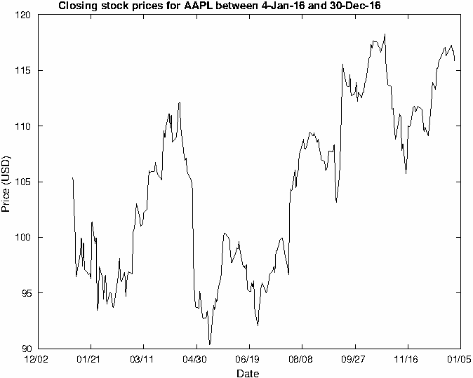
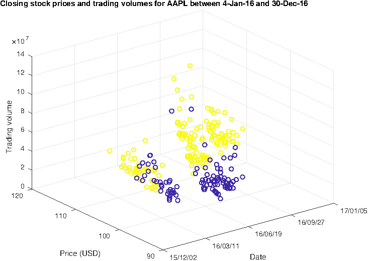
We have run the example1.m script which has downloaded Apple ('AAPL' ticker) stock data for the year 2016 and generated three plots:
- example1-2dplot.pdf : color PDF generated with the saveas function, plotting dates (x-axis) vs closing stock price (y-axis)
- example1-2dplot.eps : high quality black and white Enhanced PostScript (EPS) generated with the print function, same data as above
- example1-scatter.eps : high quality color EPS generated with the print function, showing also the trading volume (z-axis) and using different color datapoints (red) where the closing share price was above 100
The script has also used the tic/toc Matlab commands to time it's execution and we can see it took less than 2 seconds to download and process data from the Google Finance API and generate the plots.
Finally, we have closed our Matlab session and were returned to the cluster's command line prompt where we found the generated plots.
A PNG version of the latter two plots is shown below:
Further examples showing serial and parallel executions are given below in the 'Example usage of Matlab in passive mode' section.
Checking available toolboxes and license status
In order to be able to run MATLAB and specific features provided through the various MATLAB toolboxes, sufficient licenses need to
be available. The state of the licenses can be checked with the lmstat utility.
First, we will check that the license server is running (an UP status should be shown in the output of lmutil):
     (node)$> module load base/MATLAB
     (node)$> $EBROOTMATLAB/etc/glnxa64/lmutil lmstat -c $EBROOTMATLAB/licenses/network.lic
Next, we can check the total number of MATLAB licenses available (issued) and how many are used:
(node)$> $EBROOTMATLAB/etc/glnxa64/lmutil lmstat -c $EBROOTMATLAB/licenses/network.lic -f MATLAB
To check for a specific feature and its usage (e.g. the financial toolbox if we know its name):
(node)$> $EBROOTMATLAB/etc/glnxa64/lmutil lmstat -c $EBROOTMATLAB/licenses/network.lic -f Financial_toolbox
To see all available toolboxes:
(node)$> $EBROOTMATLAB/etc/glnxa64/lmutil lmstat -c $EBROOTMATLAB/licenses/network.lic -a
Checking the availability of statistics toolboxes (if we don't know the exact name, but that 'stat' is in the name):
(node)$> $EBROOTMATLAB/etc/glnxa64/lmutil lmstat -c $EBROOTMATLAB/licenses/network.lic -a | grep -i statistics
Finally, checking the available toolboxes (but with no information on the specific # of available/used licenses), can be done directly from MATLAB with the ver command.
We will load the development (experimental/testing) software set that as of June 2019 contains the newest MATLAB available (R2019a) and see this information:
     (node)$> module load swenv/default-env/devel
     (node)$> module load base/MATLAB/2019a
     (node)$> matlab -nodesktop -nodisplay
     Opening log file:  /home/users/vplugaru/java.log.16925

                             < M A T L A B (R) >
                   Copyright 1984-2019 The MathWorks, Inc.
                   R2019a (9.6.0.1072779) 64-bit (glnxa64)
                                March 8, 2019
     To get started, type doc.
     For product information, visit www.mathworks.com.

     >> ver
     -----------------------------------------------------------------------------------------------------
     MATLAB Version: 9.6.0.1072779 (R2019a)
     MATLAB License Number: 886910
     Operating System: Linux 3.10.0-693.21.1.el7.x86_64 #1 SMP Wed Mar 7 19:03:37 UTC 2018 x86_64
     Java Version: Java 1.8.0_181-b13 with Oracle Corporation Java HotSpot(TM) 64-Bit Server VM mixed mode
     -----------------------------------------------------------------------------------------------------
     MATLAB                                                Version 9.6         (R2019a)
     Simulink                                              Version 9.3         (R2019a)
     5G Toolbox                                            Version 1.1         (R2019a)
     AUTOSAR Blockset                                      Version 2.0         (R2019a)
     Aerospace Blockset                                    Version 4.1         (R2019a)
     Aerospace Toolbox                                     Version 3.1         (R2019a)
     Antenna Toolbox                                       Version 4.0         (R2019a)
     Audio Toolbox                                         Version 2.0         (R2019a)
     Automated Driving Toolbox                             Version 2.0         (R2019a)
     Bioinformatics Toolbox                                Version 4.12        (R2019a)
     Communications Toolbox                                Version 7.1         (R2019a)
     Computer Vision Toolbox                               Version 9.0         (R2019a)
     Control System Toolbox                                Version 10.6        (R2019a)
     Curve Fitting Toolbox                                 Version 3.5.9       (R2019a)
     DSP System Toolbox                                    Version 9.8         (R2019a)
     Database Toolbox                                      Version 9.1         (R2019a)
     Datafeed Toolbox                                      Version 5.8.1       (R2019a)
     Deep Learning Toolbox                                 Version 12.1        (R2019a)
     Econometrics Toolbox                                  Version 5.2         (R2019a)
     Embedded Coder                                        Version 7.2         (R2019a)
     Filter Design HDL Coder                               Version 3.1.5       (R2019a)
     Financial Instruments Toolbox                         Version 2.9         (R2019a)
     Financial Toolbox                                     Version 5.13        (R2019a)
     Fixed-Point Designer                                  Version 6.3         (R2019a)
     Fuzzy Logic Toolbox                                   Version 2.5         (R2019a)
     GPU Coder                                             Version 1.3         (R2019a)
     Global Optimization Toolbox                           Version 4.1         (R2019a)
     HDL Coder                                             Version 3.14        (R2019a)
     HDL Verifier                                          Version 5.6         (R2019a)
     Image Acquisition Toolbox                             Version 6.0         (R2019a)
     Image Processing Toolbox                              Version 10.4        (R2019a)
     Instrument Control Toolbox                            Version 4.0         (R2019a)
     LTE HDL Toolbox                                       Version 1.3         (R2019a)
     LTE Toolbox                                           Version 3.1         (R2019a)
     MATLAB Coder                                          Version 4.2         (R2019a)
     MATLAB Compiler                                       Version 7.0.1       (R2019a)
     MATLAB Compiler SDK                                   Version 6.6.1       (R2019a)
     MATLAB Report Generator                               Version 5.6         (R2019a)
     Mapping Toolbox                                       Version 4.8         (R2019a)
     Mixed-Signal Blockset                                 Version 1.0         (R2019a)
     Model Predictive Control Toolbox                      Version 6.3         (R2019a)
     Optimization Toolbox                                  Version 8.3         (R2019a)
     Parallel Computing Toolbox                            Version 7.0         (R2019a)
     Partial Differential Equation Toolbox                 Version 3.2         (R2019a)
     Phased Array System Toolbox                           Version 4.1         (R2019a)
     Powertrain Blockset                                   Version 1.5         (R2019a)
     Predictive Maintenance Toolbox                        Version 2.0         (R2019a)
     RF Blockset                                           Version 7.2         (R2019a)
     RF Toolbox                                            Version 3.6         (R2019a)
     Reinforcement Learning Toolbox                        Version 1.0         (R2019a)
     Risk Management Toolbox                               Version 1.5         (R2019a)
     Robotics System Toolbox                               Version 2.2         (R2019a)
     Robust Control Toolbox                                Version 6.6         (R2019a)
     Sensor Fusion and Tracking Toolbox                    Version 1.1         (R2019a)
     SerDes Toolbox                                        Version 1.0         (R2019a)
     Signal Processing Toolbox                             Version 8.2         (R2019a)
     SimBiology                                            Version 5.8.2       (R2019a)
     SimEvents                                             Version 5.6         (R2019a)
     Simscape                                              Version 4.6         (R2019a)
     Simscape Driveline                                    Version 2.16        (R2019a)
     Simscape Electrical                                   Version 7.1         (R2019a)
     Simscape Fluids                                       Version 2.6         (R2019a)
     Simscape Multibody                                    Version 6.1         (R2019a)
     Simulink 3D Animation                                 Version 8.2         (R2019a)
     Simulink Check                                        Version 4.3         (R2019a)
     Simulink Code Inspector                               Version 3.4         (R2019a)
     Simulink Coder                                        Version 9.1         (R2019a)
     Simulink Control Design                               Version 5.3         (R2019a)
     Simulink Coverage                                     Version 4.3         (R2019a)
     Simulink Design Optimization                          Version 3.6         (R2019a)
     Simulink Design Verifier                              Version 4.1         (R2019a)
     Simulink Report Generator                             Version 5.6         (R2019a)
     Simulink Requirements                                 Version 1.3         (R2019a)
     Simulink Test                                         Version 3.0         (R2019a)
     SoC Blockset                                          Version 1.0         (R2019a)
     Stateflow                                             Version 10.0        (R2019a)
     Statistics and Machine Learning Toolbox               Version 11.5        (R2019a)
     Symbolic Math Toolbox                                 Version 8.3         (R2019a)
     System Composer                                       Version 1.0         (R2019a)
     System Identification Toolbox                         Version 9.10        (R2019a)
     Text Analytics Toolbox                                Version 1.3         (R2019a)
     Trading Toolbox                                       Version 3.5.1       (R2019a)
     Vehicle Dynamics Blockset                             Version 1.2         (R2019a)
     Vehicle Network Toolbox                               Version 4.2         (R2019a)
     Vision HDL Toolbox                                    Version 1.8         (R2019a)
     WLAN Toolbox                                          Version 2.1         (R2019a)
     Wavelet Toolbox                                       Version 5.2         (R2019a)
Matlab execution in passive mode
For non-interactive or long executions, MATLAB can be ran in passive mode, reading all commands from an input file you provide (e.g. named INPUTFILE.m) and saving the results in an output file (e.g. named OUTPUTFILE.out), by either:
-
using redirection operators:
$> matlab -nodisplay -nosplash < INPUTFILE.m > OUTPUTFILE.out -
running the input file as a command (notice the missing '.m' extension) and copying output (as a log) to the output file:
$> matlab -nodisplay -nosplash -r INPUTFILE -logfile OUTPUTFILE.out
The second usage mode is recommended as it corresponds to the batch-mode execution. In the first case your output file will contain the '>>' characters generated by Matlab as if ran interactively, along with the results of your own commands.
However as the second usage mode runs your script as a command, it must contain the quit command at
the end in order to close Matlab, otherwise after the script has executed Matlab will stay open,
waiting for further input until the end of the walltime you set for the passive job, tying up compute
resources needlessly.
The following minimal launcher example shows how to run a serial (1 core) MATLAB script for 24 hours in passive mode:
   #!/bin/bash -l
   #SBATCH -J MATLAB
   #SBATCH -N 1
   #SBATCH -n 1
   #SBATCH -c 1
   #SBATCH --time=1-0:0:0
   #SBATCH -p batch

   module load base/MATLAB/2018a
   matlab -nodisplay -nosplash < /path/to/your/inputfile > /path/to/your/outputfile
If your MATLAB code is (ideally) using parfor constructs for parallel loops, change the -c above to e.g. 28 to use all the cores available in a compute node from the batch partition.
The most that you can get on a single node on Iris would be in the bigmem partition, which has Skylake CPUs and 112 cores per node with ~27 GB RAM/core.
Example usage of Matlab in passive mode
In this section we will use the example2.m script which shows:
- the serial execution of time consuming operations; 1 core on 1 node
- the parallel execution (based on the parfor command) and relative speedup vs serial execution, setting
the maximum number of parallel threads through environment variables; up to 1 full node
- GPU-based parallel execution; available only on GPU-enabled nodes
By default the parallel section of the script uses up to 4 threads, thus for a first test you will:
- create a launcher script called matlab-launcher.sh:
- use the launcher shown above, changing number of requested cores to 4 and a walltime of 5 minutes
- have MATLAB take its input from the example2.m m-script, and store output in example2.out
- submit the job to the scheduler with
sbatch - wait until the job completes its execution (see its status with
squeue -l -j $JOBIDand runtime details withsacct -l -j $JOBID):(access-iris)$> sbatch matlab-launcher.sh (access-iris)$> cat example2.out < M A T L A B (R) > Copyright 1984-2018 The MathWorks, Inc. R2018a (9.4.0.813654) 64-bit (glnxa64) February 23, 2018 To get started, type one of these: helpwin, helpdesk, or demo. For product information, visit www.mathworks.com. -- Will perform 200 iterations on a 1000x1000 matrix -- Serial test -- Execution time: 115.532743s. -- Parallel tests with up to 4 cores tmpJobStorageLocation = '/scratch/users/vplugaru/matlab.457594' -- Parallel test using 2 cores Starting parallel pool (parpool) using the 'local' profile ... connected to 2 workers. Parallel pool using the 'local' profile is shutting down. -- Execution time: 74.798509s. -- Execution time with overhead: 99.103444s. -- Parallel test using 4 cores Starting parallel pool (parpool) using the 'local' profile ... connected to 4 workers. Parallel pool using the 'local' profile is shutting down. -- Execution time: 39.275277s. -- Execution time with overhead: 56.273791s. -- Number of processes, parallel execution time (s), parallel execution time with overhead(s), speedup, speedup with overhead: 1.0000 115.5327 115.5327 1.0000 1.0000 2.0000 74.7985 99.1034 1.5446 1.1658 4.0000 39.2753 56.2738 2.9416 2.0530 -- GPUs not available on this system. Not running GPU-parallel test.
We will now adapt this launcher to use one of the GPU nodes of Iris, requesting part of its 28 cores and 1 of its 4 GPUs:
   #!/bin/bash -l
   #SBATCH -J MATLAB
   #SBATCH -N 1
   #SBATCH -n 1
   #SBATCH -c 7
   #SBATCH --gres=gpu:1
   #SBATCH --time=0:10:0
   #SBATCH -p gpu

   module load base/MATLAB/2018a
   matlab -nodisplay -nosplash -r example2 -logfile example2-gpu.out
Start a job with this launcher, and now you will see that the GPU test of example2.m will also be carried out. What are the 1 GPU vs CPU-only speedups?
Relative to the fast execution of the inner instruction (which calculates the eigenvalues of a matrix) the overhead given by the creation of the parallel pool and the task assignations can be quite high. You will need to be careful how you create a parallel pool as spawning the workers may not make sense if the overhead is higher compared to the computational time taken by the worker startup.
Additional work
Additional experiments are suggested:
- try the different nodes of Iris, e.g. the difference in obtained speed on Broadwell CPUs (use -C broadwell in your launcher) vs Skylake CPUs (-C skylake)
- try the scaling limits of this example, e.g. on one of the large memory nodes (use the -p bigmem bigmem partition in your launcher, with up to 112 cores)
- combine parfor with gpuArray and use the multi-GPU capabilities of Matlab (use --gres=gpu:4 for submission, you'll need to edit the example2.m file as wel)